ggtranscript is a ggplot2 extension that makes it to easy to visualize transcript structure and annotation.
Installation
# you can install the development version of ggtranscript from GitHub:
# install.packages("devtools")
devtools::install_github("dzhang32/ggtranscript")
Usage
ggtranscript introduces 5 new geoms (geom_range(), geom_half_range(), geom_intron(), geom_junction() and geom_junction_label_repel()) and several helper functions designed to facilitate the visualization of transcript structure and annotation. The following guide takes you on a quick tour of using these geoms, for a more detailed overview see the Getting Started tutorial.
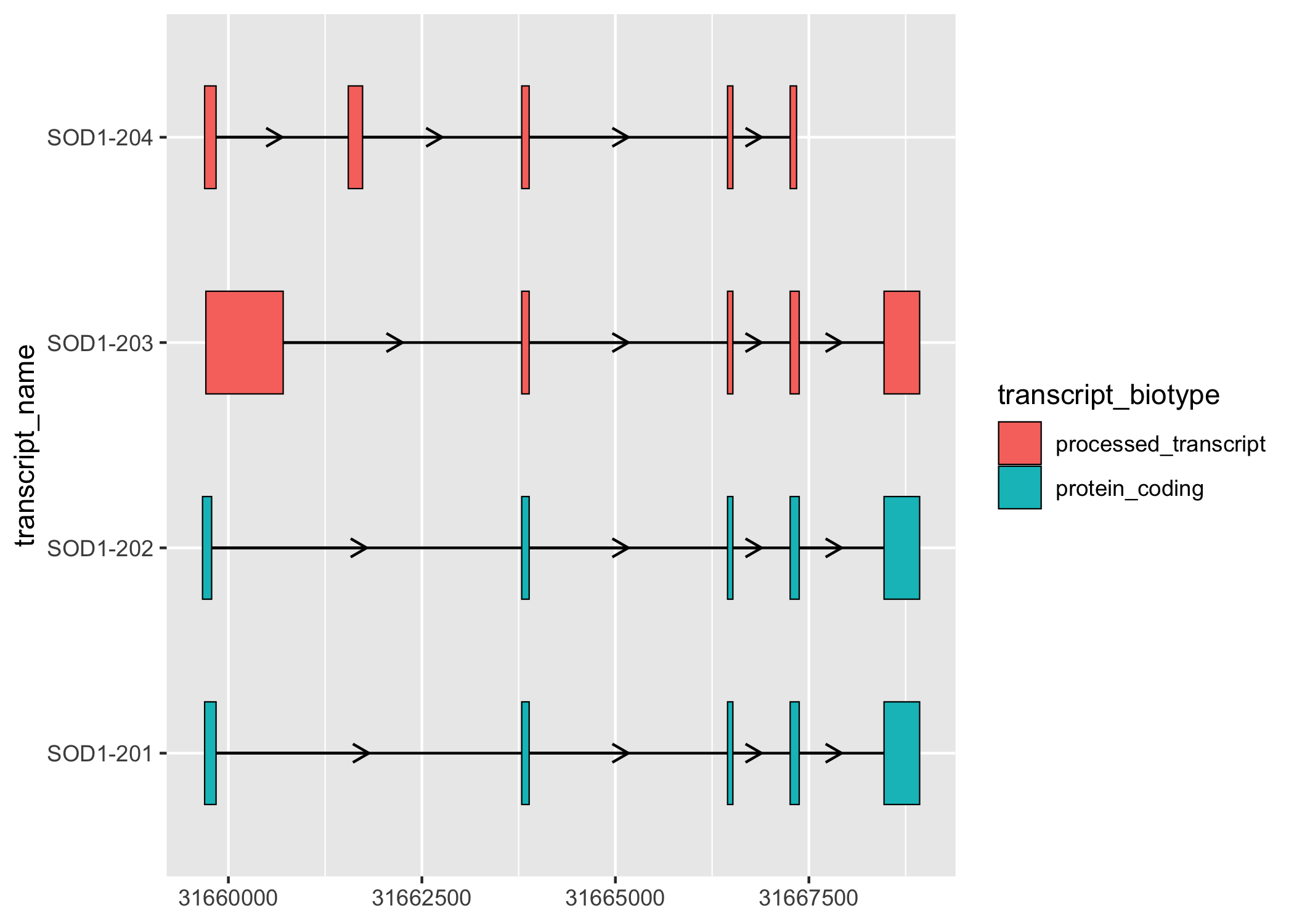
geom_range() and geom_intron() enable the plotting of exons and introns, the core components of transcript annotation. ggtranscript also provides to_intron(), which converts exon co-ordinates to the corresponding introns. Together, ggtranscript enables users to plot transcript structures with only exons as the required input and just a few lines of code.
library(magrittr)
library(dplyr)
#>
#> Attaching package: 'dplyr'
#> The following objects are masked from 'package:stats':
#>
#>     filter, lag
#> The following objects are masked from 'package:base':
#>
#>     intersect, setdiff, setequal, union
library(ggplot2)
library(ggtranscript)

# to illustrate the package's functionality
# ggtranscript includes example transcript annotation
sod1_annotation %>% head()
#> # A tibble: 6 × 8
#>   seqnames    start      end strand type        gene_name transcript_name
#>   <fct>       <int>    <int> <fct>  <fct>       <chr>     <chr>
#> 1 21       31659666 31668931 +      gene        SOD1      <NA>
#> 2 21       31659666 31668931 +      transcript  SOD1      SOD1-202
#> 3 21       31659666 31659784 +      exon        SOD1      SOD1-202
#> 4 21       31659770 31659784 +      CDS         SOD1      SOD1-202
#> 5 21       31659770 31659772 +      start_codon SOD1      SOD1-202
#> 6 21       31663790 31663886 +      exon        SOD1      SOD1-202
#> # ℹ 1 more variable: transcript_biotype <chr>

# extract exons
sod1_exons <- sod1_annotation %>% dplyr::filter(type == "exon")

sod1_exons %>%
    ggplot(aes(
        xstart = start,
        xend = end,
        y = transcript_name
    )) +
    geom_range(
        aes(fill = transcript_biotype)
    ) +
    geom_intron(
        data = to_intron(sod1_exons, "transcript_name"),
        aes(strand = strand)
    )
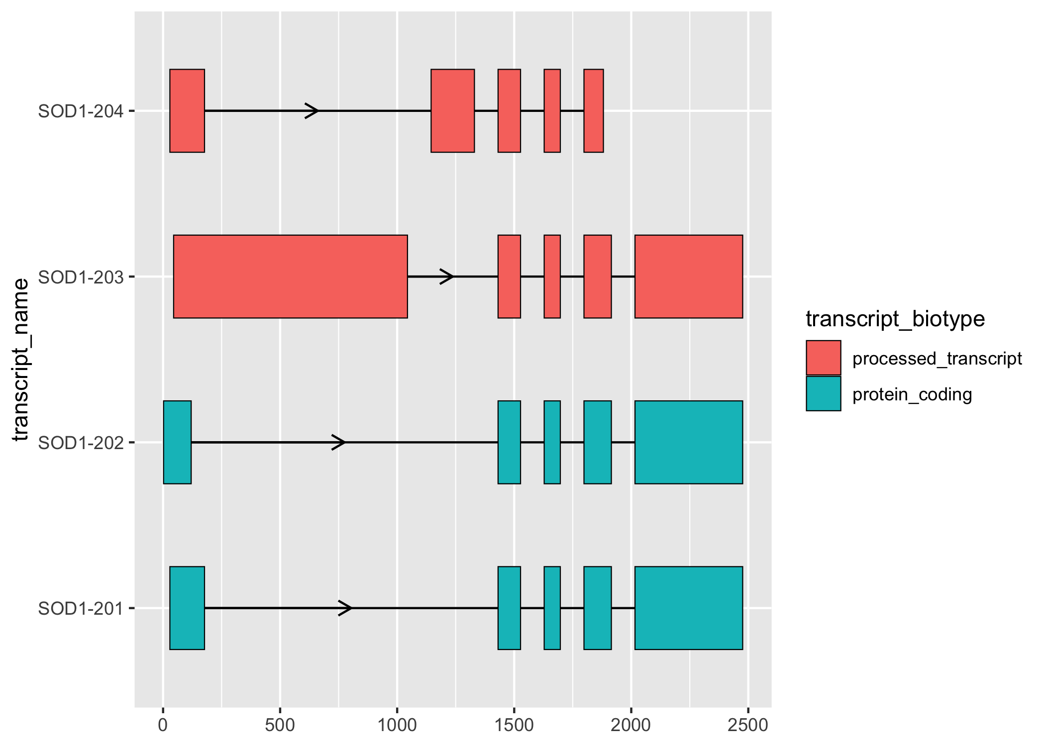
ggtranscript provides the helper function shorten_gaps(), which reduces the size of the gaps. shorten_gaps() then rescales the exon and intron co-ordinates to preserve the original exon alignment. This allows you to hone in the differences in the exonic structure, which can be particularly useful if the transcript has relatively long introns.
sod1_rescaled <- shorten_gaps(
  sod1_exons,
  to_intron(sod1_exons, "transcript_name"),
  group_var = "transcript_name"
  )

sod1_rescaled %>%
    dplyr::filter(type == "exon") %>%
    ggplot(aes(
        xstart = start,
        xend = end,
        y = transcript_name
    )) +
    geom_range(
      aes(fill = transcript_biotype)
    ) +
    geom_intron(
        data = sod1_rescaled %>% dplyr::filter(type == "intron"),
        arrow.min.intron.length = 200
    )
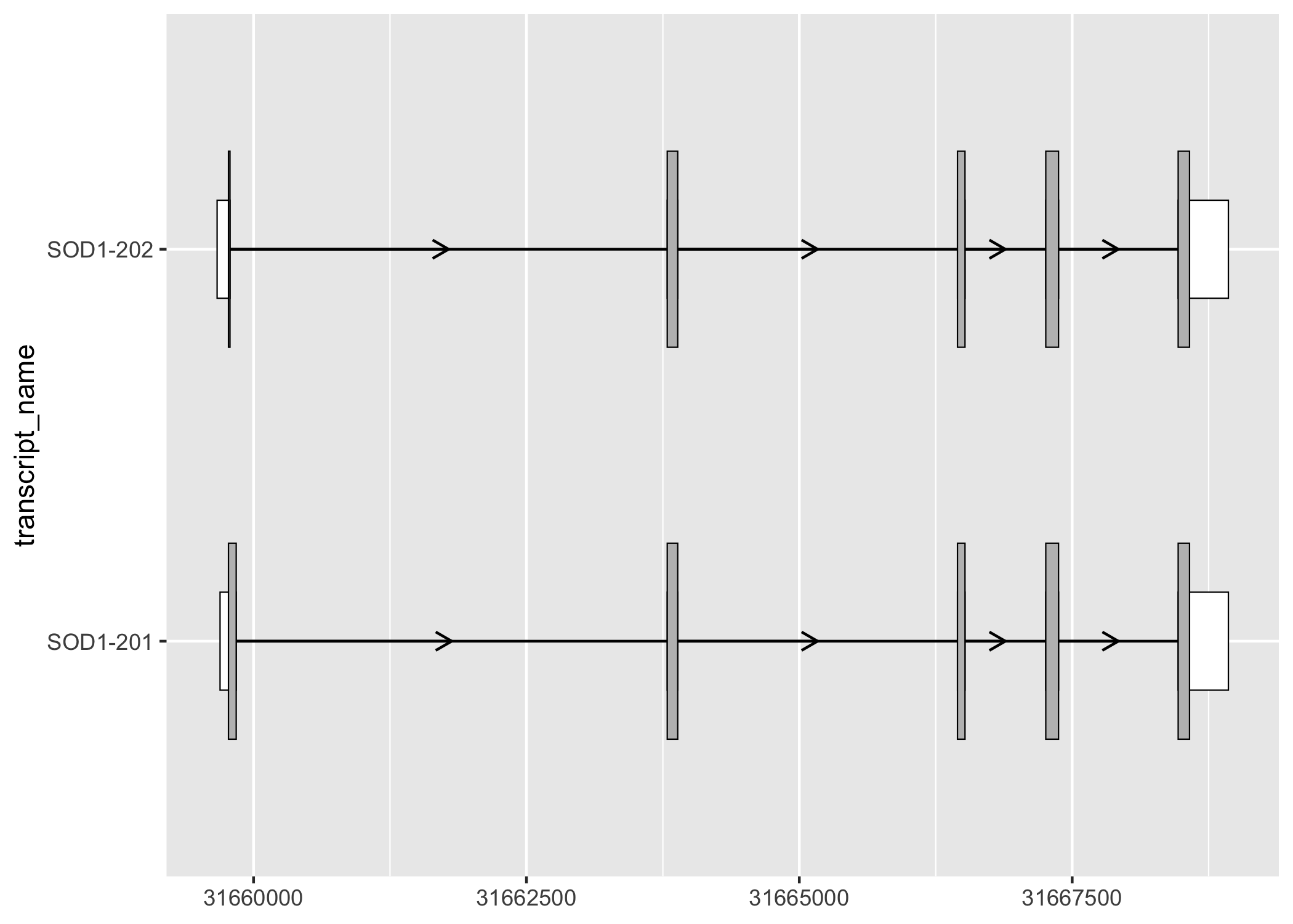
geom_range() can be used for any range-based genomic annotation. For example, when plotting protein-coding transcripts, users may find it helpful to visually distinguish the coding segments from UTRs.
# filter for only exons from protein coding transcripts
sod1_exons_prot_cod <- sod1_exons %>%
    dplyr::filter(transcript_biotype == "protein_coding")

# obtain cds
sod1_cds <- sod1_annotation %>% dplyr::filter(type == "CDS")

sod1_exons_prot_cod %>%
    ggplot(aes(
        xstart = start,
        xend = end,
        y = transcript_name
    )) +
    geom_range(
        fill = "white",
        height = 0.25
    ) +
    geom_range(
        data = sod1_cds
    ) +
    geom_intron(
        data = to_intron(sod1_exons_prot_cod, "transcript_name"),
        aes(strand = strand),
        arrow.min.intron.length = 500,
    )
geom_half_range() takes advantage of the vertical symmetry of transcript annotation by plotting only half of a range on the top or bottom of a transcript structure. One use case of geom_half_range() is to visualize the differences between transcript structure more clearly.
# extract exons and cds for the two transcripts to be compared
sod1_201_exons <- sod1_exons %>% dplyr::filter(transcript_name == "SOD1-201")
sod1_201_cds <- sod1_cds %>% dplyr::filter(transcript_name == "SOD1-201")
sod1_202_exons <- sod1_exons %>% dplyr::filter(transcript_name == "SOD1-202")
sod1_202_cds <- sod1_cds %>% dplyr::filter(transcript_name == "SOD1-202")

sod1_201_202_plot <- sod1_201_exons %>%
    ggplot(aes(
        xstart = start,
        xend = end,
        y = "SOD1-201/202"
    )) +
    geom_half_range(
        fill = "white",
        height = 0.125
    ) +
    geom_half_range(
        data = sod1_201_cds
    ) +
    geom_intron(
        data = to_intron(sod1_201_exons, "transcript_name")
    ) +
    geom_half_range(
        data = sod1_202_exons,
        range.orientation = "top",
        fill = "white",
        height = 0.125
    ) +
    geom_half_range(
        data = sod1_202_cds,
        range.orientation = "top",
        fill = "purple"
    ) +
    geom_intron(
        data = to_intron(sod1_202_exons, "transcript_name")
    )

sod1_201_202_plot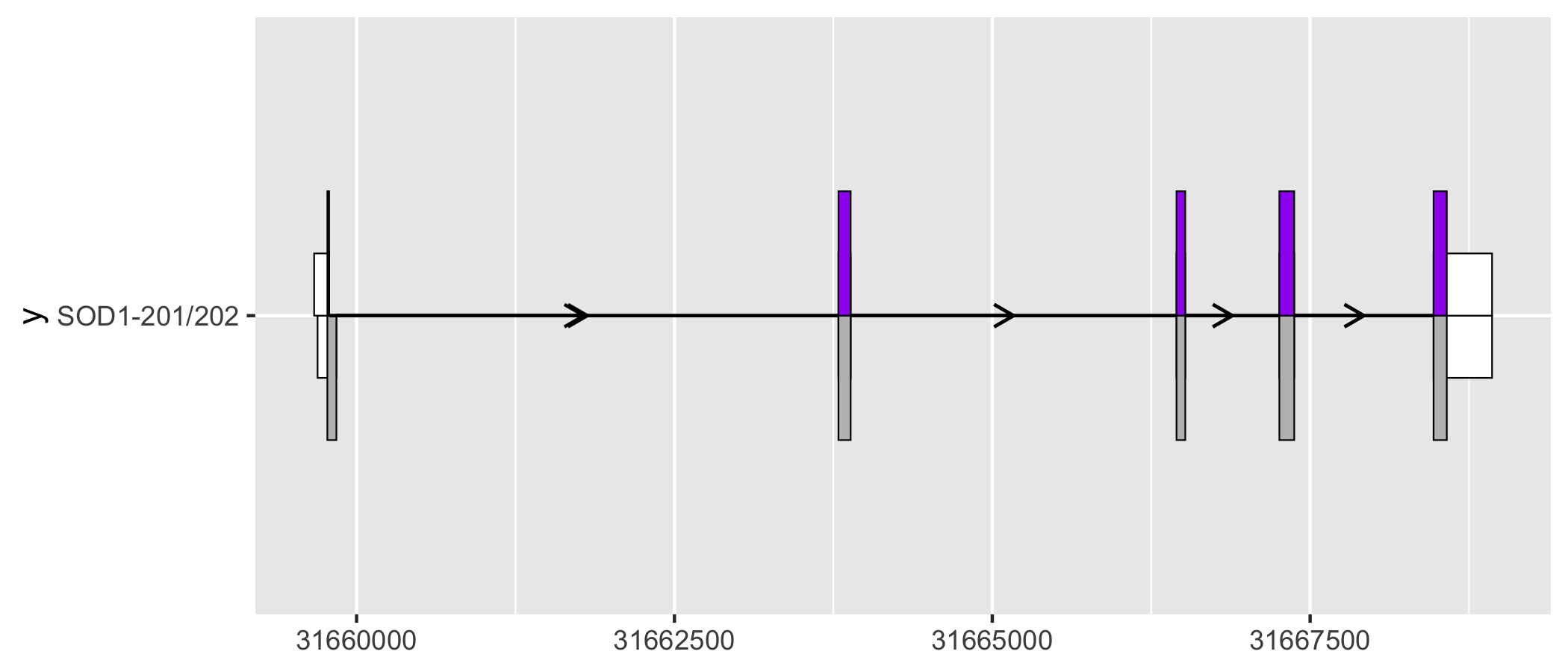
As a ggplot2 extension, ggtranscript inherits the the familiarity and functionality of ggplot2. For instance, by leveraging coord_cartesian() users can zoom in on regions of interest.
sod1_201_202_plot + coord_cartesian(xlim = c(31659500, 31660000))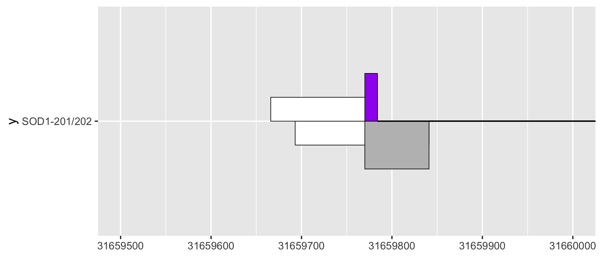
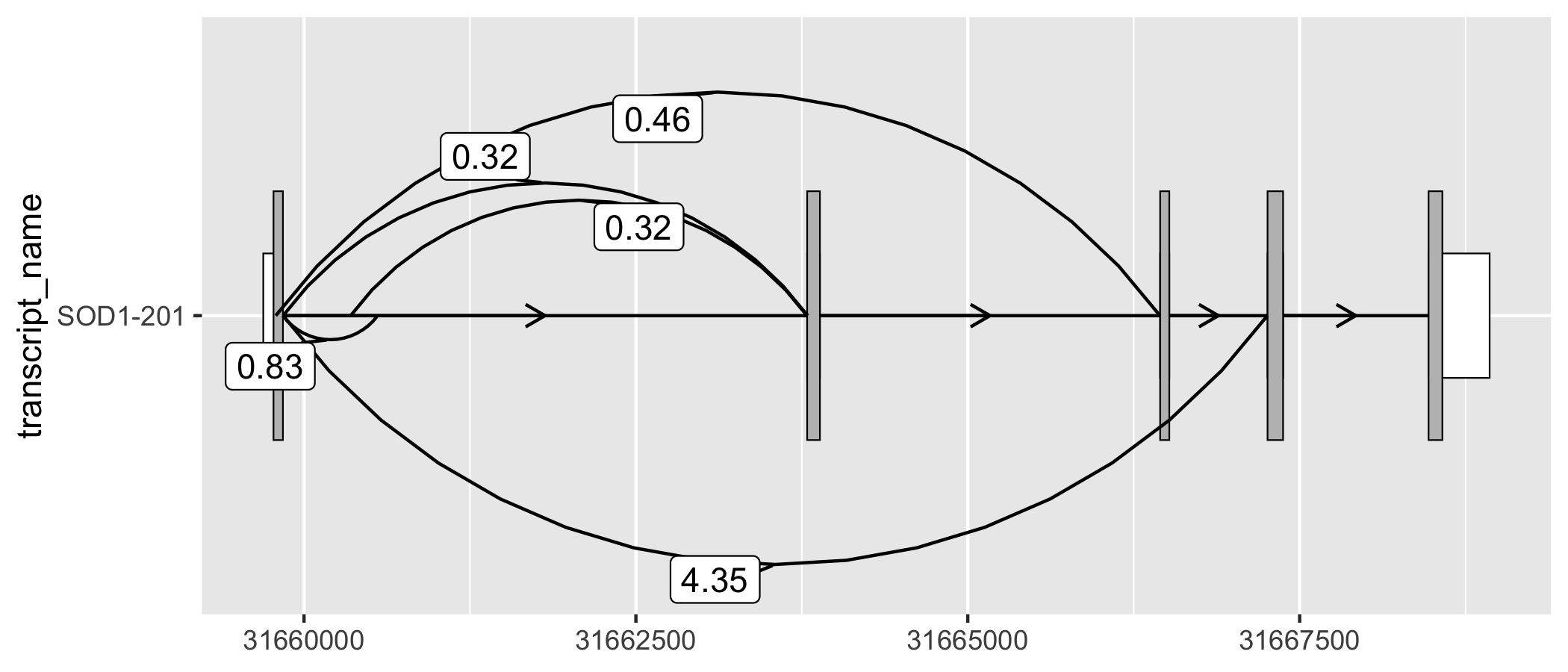
geom_junction() enables to plotting of junction curves, which can be overlaid across transcript structures. geom_junction_label_repel() adds a label to junction curves, which can often be useful to mark junctions with a metric of their usage such as read counts.
# ggtranscript includes a set of example (unannotated) junctions
# originating from GTEx and downloaded via the Bioconductor package snapcount
sod1_junctions
#> # A tibble: 5 × 5
#>   seqnames    start      end strand mean_count
#>   <fct>       <int>    <int> <fct>       <dbl>
#> 1 chr21    31659787 31666448 +           0.463
#> 2 chr21    31659842 31660554 +           0.831
#> 3 chr21    31659842 31663794 +           0.316
#> 4 chr21    31659842 31667257 +           4.35
#> 5 chr21    31660351 31663789 +           0.324

# add transcript_name to junctions for plotting
sod1_junctions <- sod1_junctions %>%
    dplyr::mutate(transcript_name = "SOD1-201")

sod1_201_exons %>%
  ggplot(aes(
    xstart = start,
    xend = end,
    y = transcript_name
  )) +
  geom_range(
    fill = "white",
    height = 0.25
  ) +
  geom_range(
    data = sod1_201_cds
  ) +
  geom_intron(
    data = to_intron(sod1_201_exons, "transcript_name")
  ) +
  geom_junction(
    data = sod1_junctions,
    junction.y.max = 0.5
  ) +
  geom_junction_label_repel(
    data = sod1_junctions,
    aes(label = round(mean_count, 2)),
    junction.y.max = 0.5
  )
Alternatively, users may prefer to map junction read counts to the thickness of the junction curves. As a ggplot2 extension, this can be done intuitively by modifying the size aes() of geom_junction(). In addition, by modifying ggplot2 scales and themes, users can easily create informative, publication-ready plots.
sod1_201_exons %>%
  ggplot(aes(
    xstart = start,
    xend = end,
    y = transcript_name
  )) +
  geom_range(
    fill = "white",
    height = 0.25
  ) +
  geom_range(
    data = sod1_201_cds
  ) +
  geom_intron(
    data = to_intron(sod1_201_exons, "transcript_name")
  ) +
  geom_junction(
    data = sod1_junctions,
    aes(size = mean_count),
    junction.y.max = 0.5,
    ncp = 30,
    colour = "purple"
  ) +
  scale_size_continuous(range = c(0.1, 1), guide = "none") +
  xlab("Genomic position (chr21)") +
  ylab("Transcript name") +
  theme_bw()
#> Warning: Using `size` aesthetic for lines was deprecated in ggplot2 3.4.0.
#> ℹ Please use `linewidth` instead.
#> This warning is displayed once every 8 hours.
#> Call `lifecycle::last_lifecycle_warnings()` to see where this warning was
#> generated.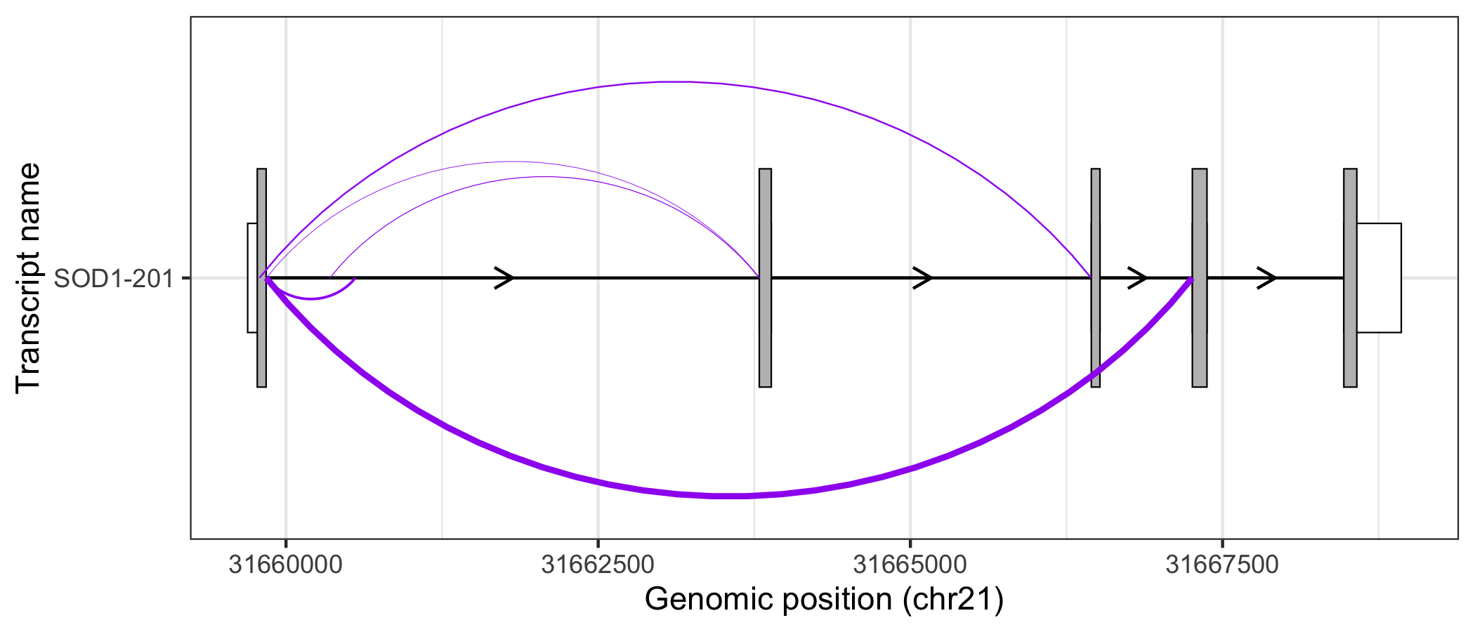
Citation
citation("ggtranscript")
#> To cite package 'ggtranscript' in publications use:
#>
#>   Gustavsson EK, Zhang D, Reynolds RH, Garcia-Ruiz S, Ryten M (2022).
#>   "ggtranscript: an R package for the visualization and interpretation
#>   of transcript isoforms using ggplot2." _Bioinformatics_.
#>   doi:10.1093/bioinformatics/btac409
#>   <https://doi.org/10.1093/bioinformatics/btac409>,
#>   <https://academic.oup.com/bioinformatics/article/38/15/3844/6617821>.
#>
#> A BibTeX entry for LaTeX users is
#>
#>   @Article{,
#>     title = {ggtranscript: an R package for the visualization and interpretation of transcript isoforms using ggplot2},
#>     author = {Emil K Gustavsson and David Zhang and Regina H Reynolds and Sonia Garcia-Ruiz and Mina Ryten},
#>     year = {2022},
#>     journal = {Bioinformatics},
#>     doi = {https://doi.org/10.1093/bioinformatics/btac409},
#>     url = {https://academic.oup.com/bioinformatics/article/38/15/3844/6617821},
#>   }