Plot genomic ranges

geom_range() and geom_half_range() draw tiles that are designed to represent range-based genomic features, such as exons. In combination with geom_intron(), these geoms form the core components for visualizing transcript structures.

Usage

geom_range(
  mapping = NULL,
  data = NULL,
  stat = "identity",
  position = "identity",
  ...,
  vjust = NULL,
  linejoin = "mitre",
  na.rm = FALSE,
  show.legend = NA,
  inherit.aes = TRUE
)

geom_half_range(
  mapping = NULL,
  data = NULL,
  stat = "identity",
  position = "identity",
  ...,
  range.orientation = "bottom",
  linejoin = "mitre",
  na.rm = FALSE,
  show.legend = NA,
  inherit.aes = TRUE
)

Arguments

mapping

Set of aesthetic mappings created by aes() or aes_(). If specified and inherit.aes = TRUE (the default), it is combined with the default mapping at the top level of the plot. You must supply mapping if there is no plot mapping.

data

The data to be displayed in this layer. There are three options:

If NULL, the default, the data is inherited from the plot data as specified in the call to ggplot().

A data.frame, or other object, will override the plot data. All objects will be fortified to produce a data frame. See fortify() for which variables will be created.

A function will be called with a single argument, the plot data. The return value must be a data.frame, and will be used as the layer data. A function can be created from a formula (e.g. ~ head(.x, 10)).

stat

The statistical transformation to use on the data for this layer, as a string.

position

Position adjustment, either as a string, or the result of a call to a position adjustment function.

...

Other arguments passed on to layer(). These are often aesthetics, used to set an aesthetic to a fixed value, like colour = "red" or size = 3. They may also be parameters to the paired geom/stat.

vjust

horizontal and vertical justification of the grob. Each justification value should be a number between 0 and 1. Defaults to 0.5 for both, centering each pixel over its data location.

linejoin

Line join style (round, mitre, bevel).

na.rm

If FALSE, the default, missing values are removed with a warning. If TRUE, missing values are silently removed.

show.legend

logical. Should this layer be included in the legends? NA, the default, includes if any aesthetics are mapped. FALSE never includes, and TRUE always includes. It can also be a named logical vector to finely select the aesthetics to display.

inherit.aes

If FALSE, overrides the default aesthetics, rather than combining with them. This is most useful for helper functions that define both data and aesthetics and shouldn't inherit behaviour from the default plot specification, e.g. borders().

range.orientation

character() one of "top" or "bottom", specifying where the half ranges will be plotted with respect to each transcript (y).

Value

the return value of a geom_* function is not intended to be directly handled by users. Therefore, geom_* functions should never be executed in isolation, rather used in combination with a ggplot2::ggplot() call.

Details

geom_range() and geom_half_range() require the following aes(); xstart, xend and y (e.g. transcript name). geom_half_range() takes advantage of the vertical symmetry of transcript annotation by plotting only half of a range on the top or bottom of a transcript structure. This can be useful for comparing between two transcripts or free up plotting space for other transcript annotations (e.g. geom_junction()).

Examples

library(magrittr)
library(ggplot2)

# to illustrate the package's functionality
# ggtranscript includes example transcript annotation
sod1_annotation %>% head()
#> # A tibble: 6 × 8
#>   seqnames  start    end strand type  gene_name transcript_name transcript_biot…
#>   <fct>     <int>  <int> <fct>  <fct> <chr>     <chr>           <chr>           
#> 1 21       3.17e7 3.17e7 +      gene  SOD1      NA              NA              
#> 2 21       3.17e7 3.17e7 +      tran… SOD1      SOD1-202        protein_coding  
#> 3 21       3.17e7 3.17e7 +      exon  SOD1      SOD1-202        protein_coding  
#> 4 21       3.17e7 3.17e7 +      CDS   SOD1      SOD1-202        protein_coding  
#> 5 21       3.17e7 3.17e7 +      star… SOD1      SOD1-202        protein_coding  
#> 6 21       3.17e7 3.17e7 +      exon  SOD1      SOD1-202        protein_coding  

# extract exons
sod1_exons <- sod1_annotation %>% dplyr::filter(type == "exon")
sod1_exons %>% head()
#> # A tibble: 6 × 8
#>   seqnames  start    end strand type  gene_name transcript_name transcript_biot…
#>   <fct>     <int>  <int> <fct>  <fct> <chr>     <chr>           <chr>           
#> 1 21       3.17e7 3.17e7 +      exon  SOD1      SOD1-202        protein_coding  
#> 2 21       3.17e7 3.17e7 +      exon  SOD1      SOD1-202        protein_coding  
#> 3 21       3.17e7 3.17e7 +      exon  SOD1      SOD1-202        protein_coding  
#> 4 21       3.17e7 3.17e7 +      exon  SOD1      SOD1-202        protein_coding  
#> 5 21       3.17e7 3.17e7 +      exon  SOD1      SOD1-202        protein_coding  
#> 6 21       3.17e7 3.17e7 +      exon  SOD1      SOD1-204        processed_trans…

base <- sod1_exons %>%
    ggplot(aes(
        xstart = start,
        xend = end,
        y = transcript_name
    ))

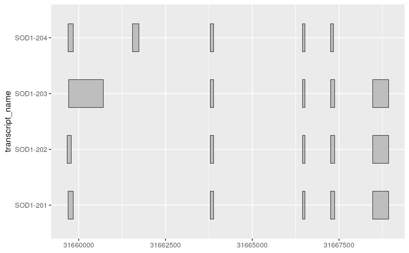
# geom_range() is designed to visualise range-based annotation such as exons
base + geom_range()


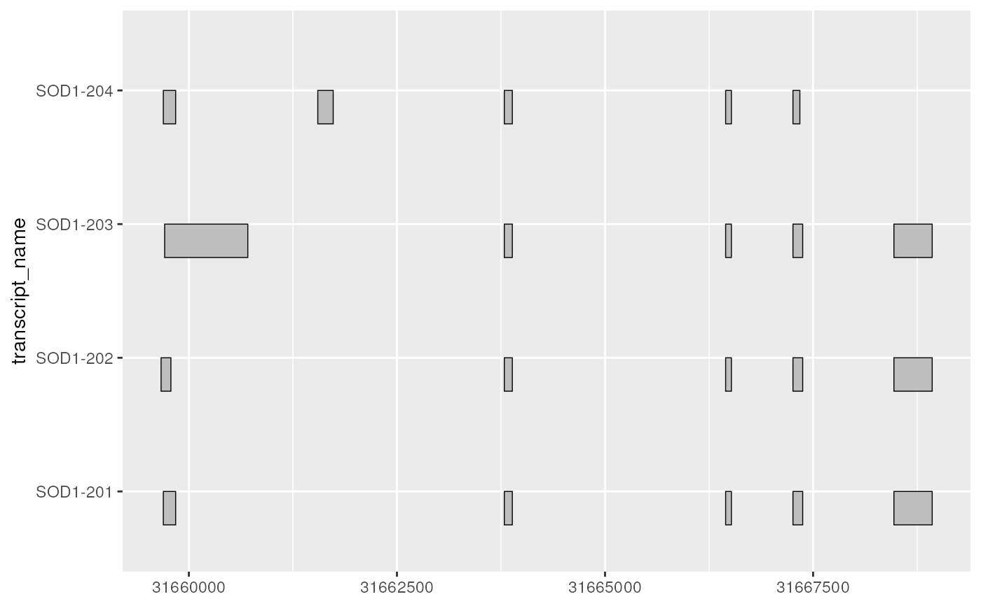
# geom_half_range() allows users to plot half ranges
# on the top or bottom of the transcript
base + geom_half_range()


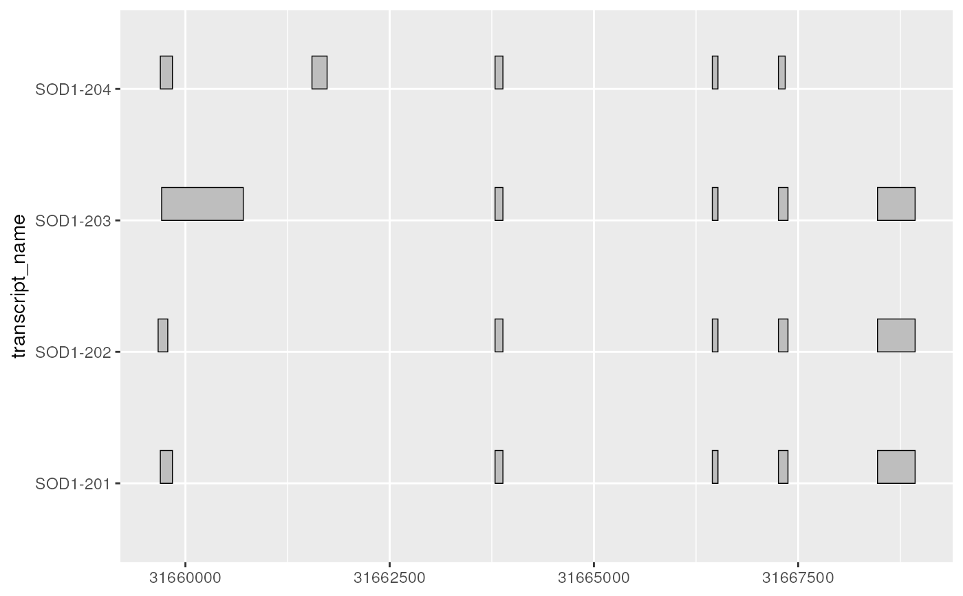
# where the half ranges are plotted can be adjusted using range.orientation
base + geom_half_range(range.orientation = "top")


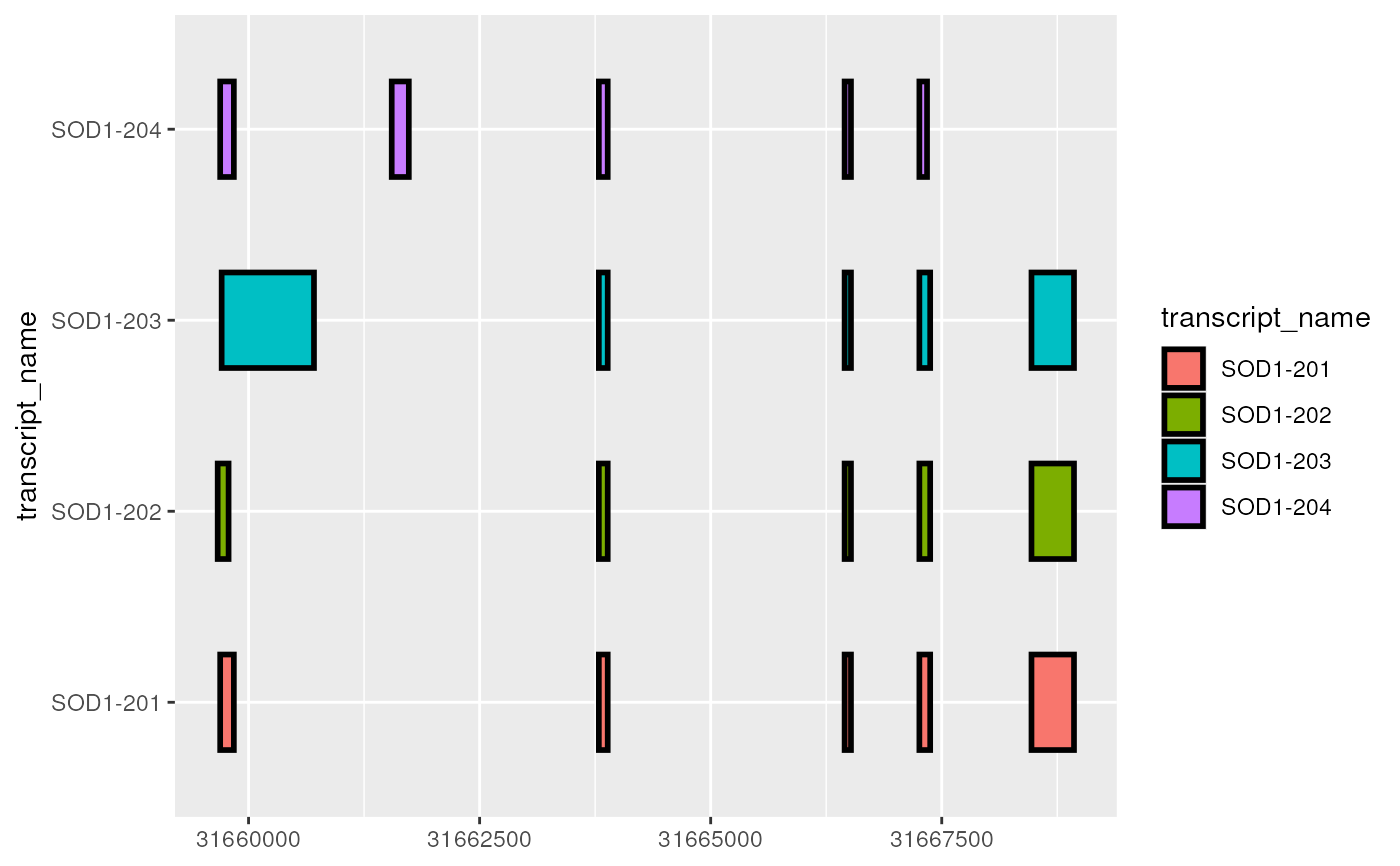
# as a ggplot2 extension, ggtranscript geoms inherit the
# the functionality from the parameters and aesthetics in ggplot2
base + geom_range(
    aes(fill = transcript_name),
    size = 1
)


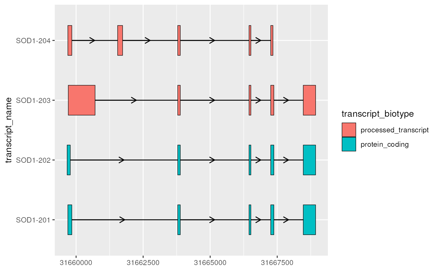
# together, geom_range() and geom_intron() are designed to visualize
# the core components of transcript annotation
base + geom_range(
    aes(fill = transcript_biotype)
) +
    geom_intron(
        data = to_intron(sod1_exons, "transcript_name")
    )


# for protein coding transcripts
# geom_range() be useful for visualizing UTRs that lie outside of the CDS
sod1_exons_prot_coding <- sod1_exons %>%
    dplyr::filter(transcript_biotype == "protein_coding")

# extract cds
sod1_cds <- sod1_annotation %>%
    dplyr::filter(type == "CDS")

sod1_exons_prot_coding %>%
    ggplot(aes(
        xstart = start,
        xend = end,
        y = transcript_name
    )) +
    geom_range(
        fill = "white",
        height = 0.25
    ) +
    geom_range(
        data = sod1_cds
    ) +
    geom_intron(
        data = to_intron(sod1_exons_prot_coding, "transcript_name")
    )


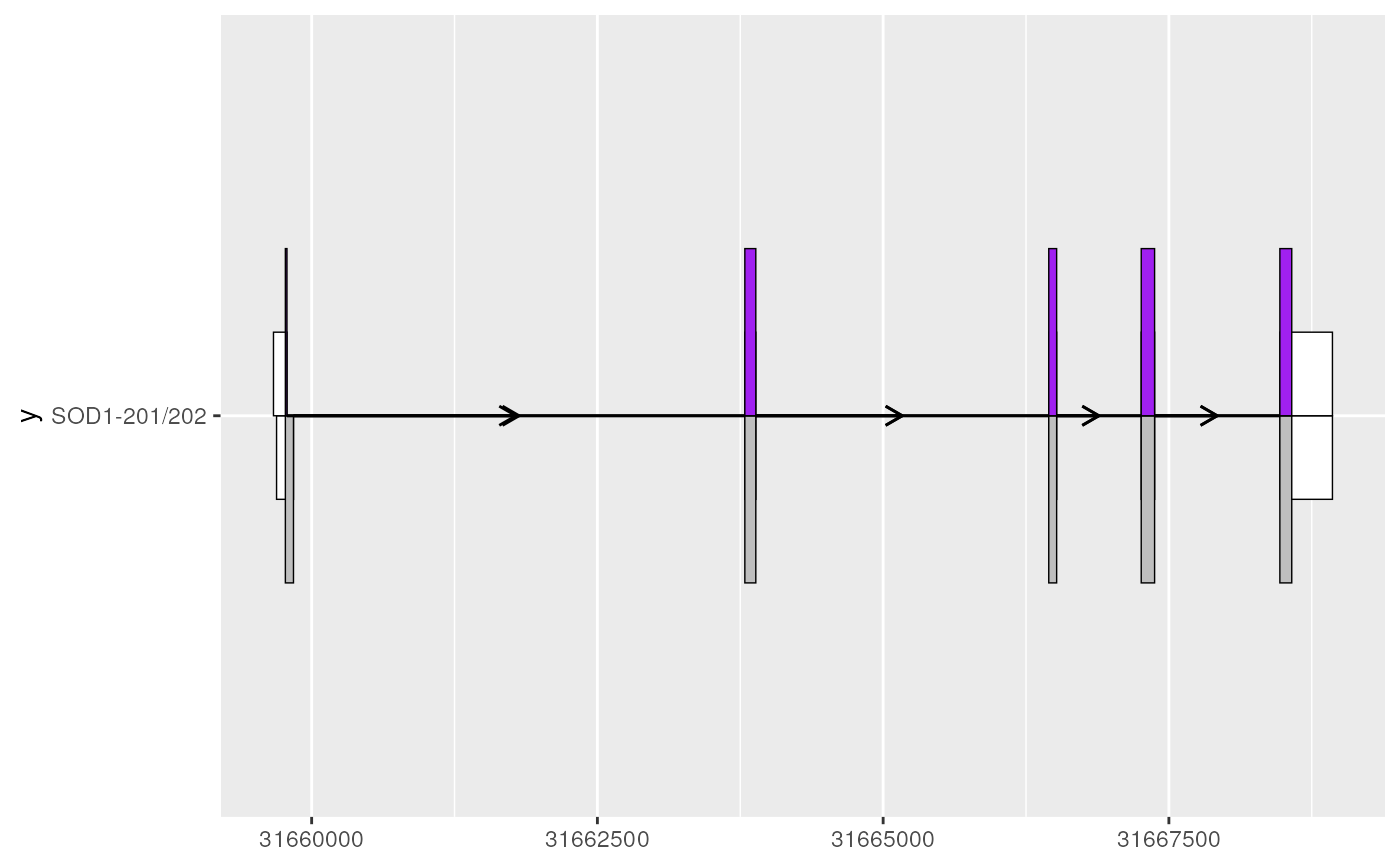
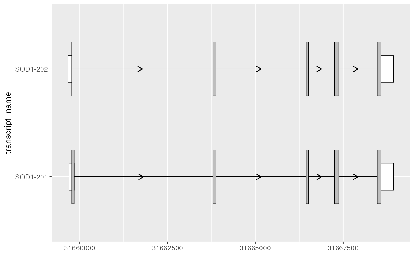# geom_half_range() can be useful for comparing between two transcripts
# enabling visualization of one transcript on the top, other on the bottom
sod1_201_exons <- sod1_exons %>% dplyr::filter(transcript_name == "SOD1-201")
sod1_201_cds <- sod1_cds %>% dplyr::filter(transcript_name == "SOD1-201")
sod1_202_exons <- sod1_exons %>% dplyr::filter(transcript_name == "SOD1-202")
sod1_202_cds <- sod1_cds %>% dplyr::filter(transcript_name == "SOD1-202")

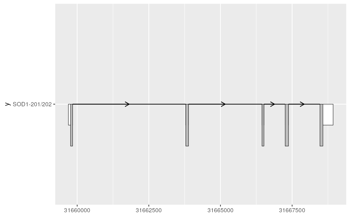
sod1_201_plot <- sod1_201_exons %>%
    ggplot(aes(
        xstart = start,
        xend = end,
        y = "SOD1-201/202"
    )) +
    geom_half_range(
        fill = "white",
        height = 0.125
    ) +
    geom_half_range(
        data = sod1_201_cds
    ) +
    geom_intron(
        data = to_intron(sod1_201_exons, "transcript_name")
    )

sod1_201_plot


sod1_201_202_plot <- sod1_201_plot +
    geom_half_range(
        data = sod1_202_exons,
        range.orientation = "top",
        fill = "white",
        height = 0.125
    ) +
    geom_half_range(
        data = sod1_202_cds,
        range.orientation = "top",
        fill = "purple"
    ) +
    geom_intron(
        data = to_intron(sod1_202_exons, "transcript_name")
    )

sod1_201_202_plot


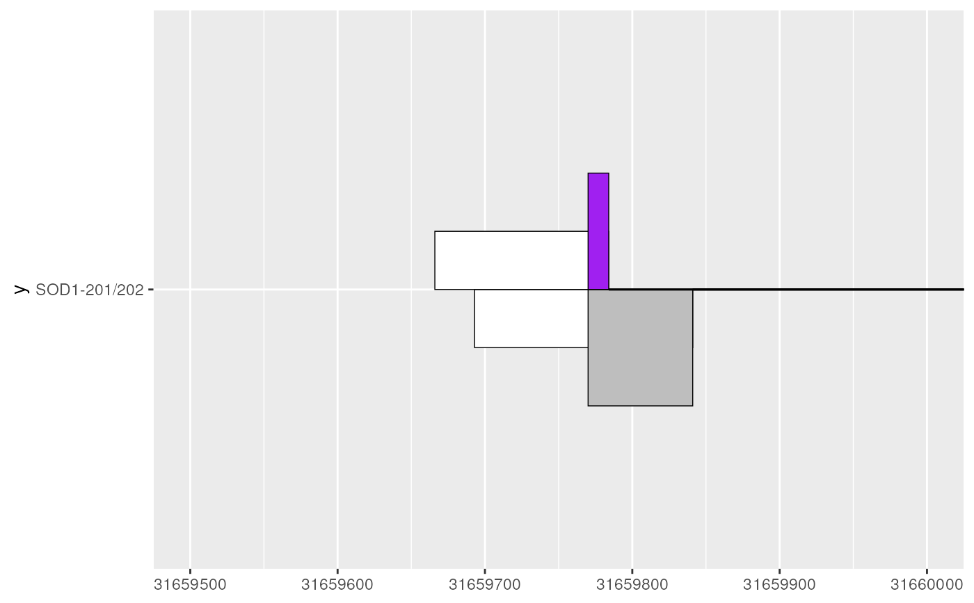
# leveraging existing ggplot2 functionality via e.g. coord_cartesian()
# can be useful to zoom in on areas of interest
sod1_201_202_plot + coord_cartesian(xlim = c(31659500, 31660000))