Convert exon co-ordinates to introns — to

Given a set of exons, to_intron() will return the corresponding introns.

Usage

to_intron(exons, group_var = NULL)

Arguments

exons: data.frame() contains exons which can originate from multiple transcripts differentiated by group_var.
group_var: character() if input data originates from more than 1 transcript, group_var must specify the column that differentiates transcripts (e.g. "transcript_id").

Value

data.frame() contains the intron co-ordinates.

Details

It is important to note that, for visualization purposes, to_intron() defines introns precisely as the exon boundaries, rather than the intron start/end being (exon end + 1)/(exon start - 1).

Examples

library(magrittr)
library(ggplot2)

# to illustrate the package's functionality
# ggtranscript includes example transcript annotation
sod1_annotation %>% head()
#> # A tibble: 6 × 8
#>   seqnames    start      end strand type        gene_name transcript_name
#>   <fct>       <int>    <int> <fct>  <fct>       <chr>     <chr>          
#> 1 21       31659666 31668931 +      gene        SOD1      NA             
#> 2 21       31659666 31668931 +      transcript  SOD1      SOD1-202       
#> 3 21       31659666 31659784 +      exon        SOD1      SOD1-202       
#> 4 21       31659770 31659784 +      CDS         SOD1      SOD1-202       
#> 5 21       31659770 31659772 +      start_codon SOD1      SOD1-202       
#> 6 21       31663790 31663886 +      exon        SOD1      SOD1-202       
#> # ℹ 1 more variable: transcript_biotype <chr>

# extract exons
sod1_exons <- sod1_annotation %>% dplyr::filter(type == "exon")
sod1_exons %>% head()
#> # A tibble: 6 × 8
#>   seqnames    start      end strand type  gene_name transcript_name
#>   <fct>       <int>    <int> <fct>  <fct> <chr>     <chr>          
#> 1 21       31659666 31659784 +      exon  SOD1      SOD1-202       
#> 2 21       31663790 31663886 +      exon  SOD1      SOD1-202       
#> 3 21       31666449 31666518 +      exon  SOD1      SOD1-202       
#> 4 21       31667258 31667375 +      exon  SOD1      SOD1-202       
#> 5 21       31668471 31668931 +      exon  SOD1      SOD1-202       
#> 6 21       31659693 31659841 +      exon  SOD1      SOD1-204       
#> # ℹ 1 more variable: transcript_biotype <chr>

# to_intron() is a helper function included in ggtranscript
# which is useful for converting exon co-ordinates to introns
sod1_introns <- sod1_exons %>% to_intron(group_var = "transcript_name")
sod1_introns %>% head()
#> # A tibble: 6 × 8
#>   seqnames strand type   gene_name transcript_name transcript_biotype      start
#>   <fct>    <fct>  <chr>  <chr>     <chr>           <chr>                   <int>
#> 1 21       +      intron SOD1      SOD1-204        processed_transcript 31659841
#> 2 21       +      intron SOD1      SOD1-202        protein_coding       31659784
#> 3 21       +      intron SOD1      SOD1-204        processed_transcript 31661734
#> 4 21       +      intron SOD1      SOD1-201        protein_coding       31659841
#> 5 21       +      intron SOD1      SOD1-203        processed_transcript 31660708
#> 6 21       +      intron SOD1      SOD1-202        protein_coding       31663886
#> # ℹ 1 more variable: end <int>

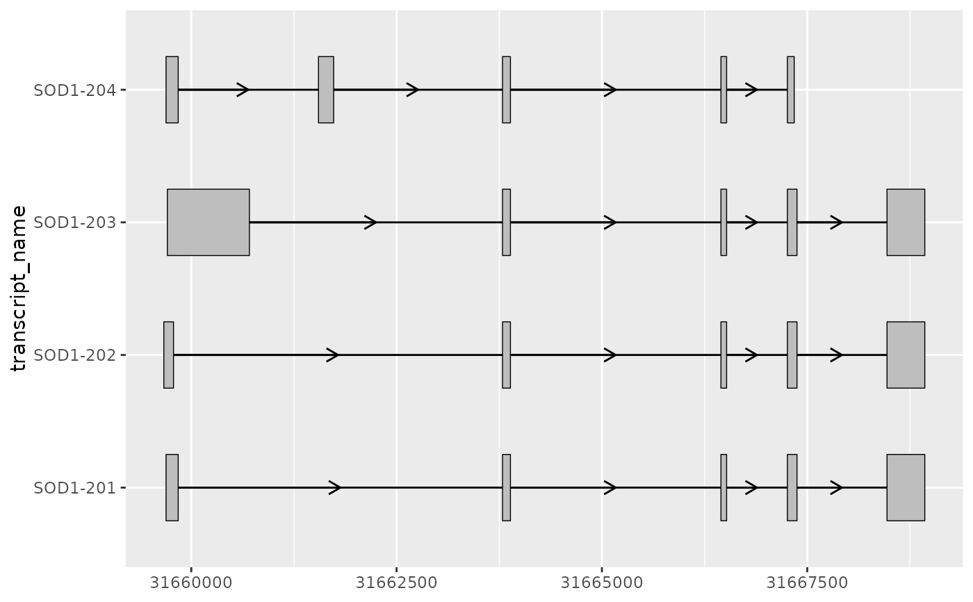
# this can be particular useful when combined with
# geom_range() and geom_intron()
# to visualize the core components of transcript annotation
sod1_exons %>%
    ggplot(aes(
        xstart = start,
        xend = end,
        y = transcript_name
    )) +
    geom_range() +
    geom_intron(
        data = to_intron(sod1_exons, "transcript_name")
    )